Build Your First Computer Vision Project — Dog Breed Classification

14 Oct 2019 in Blog

Get started building your first computer vision project in less than 30 minutes.

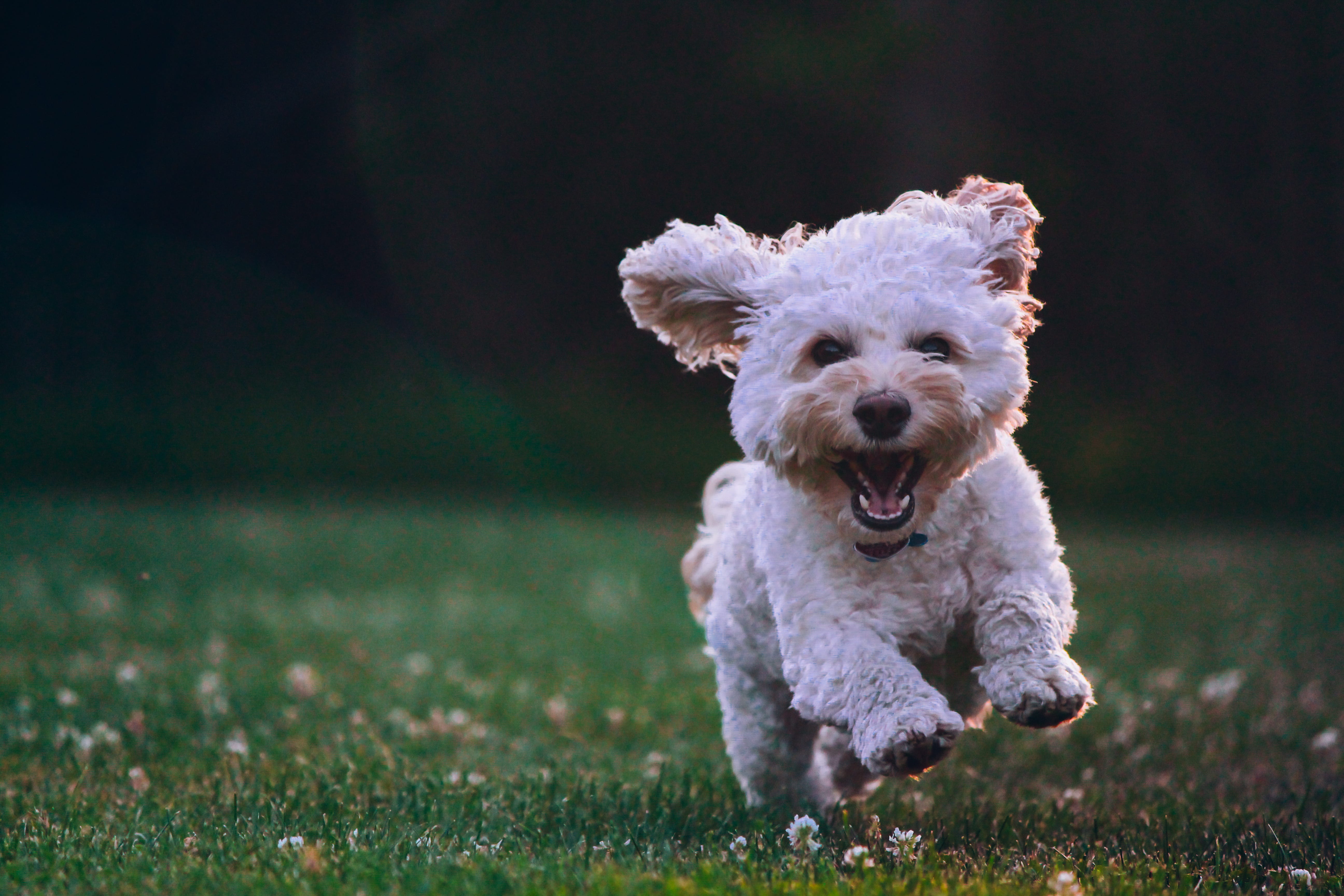
For us, humans, it is pretty easy to tell one dog breed from another. That is if you are talking about 10–20 popular dog breeds. When we are talking about more than 100 kinds of dogs, it is an entirely different story. For a human to correctly and consistently classify a large number of breeds, we need a different approach than just pure memorization. We need to start extracting “features” that correspond to different breeds such as fur color, ear shape, facial shape, tail length, etc. Even then, we need to memorize what breed has what features, and it’s not an easy or fun task.

Image credit: It is hard to classify a large number of dog breeds

Humans having difficulties identifying a large number of species is a perfect example of situations where computers are better than us. This is not to say that Skynet is coming to kill us all; I believe that we should not worry about that just yet. Instead of machines replacing humans in the workforce, many believe that a hybrid approach of the two races working together can outperform any single race working alone. You can read more about the topic in the book titled Machine, Platform, Crowd by Andrew McAfee.

In this project, I will walk you through the steps to build and train a convolutional neural network (CNN) that will classify 133 different dog breeds. This project is part of my Data scientist Nanodegree, and you can find out more about it here. The code for this project is available on my GitHub repo, make sure that you install the required packages if you want to follow along.

What you need to know

How computer understand an image

We are very good at recognizing things thanks to millions of years of evolution that went into perfecting our eyes and brains for vision capability. A computer “sees” an image as a series of numbers. A pixel on your screen is represented as three numbers from 0 to 255. Each number is represented as the intensity of red, green, and blue. A 1024x768 picture can be expressed as a 1024x768x3 matrix equivalent to a series of 239,616 numbers.

Image credit: Image represented as numbers

Traditionally, it’s tough for a computer to recognize or classify an object in an image. With the recent advancements in computing power and neural network research, computers can now have human-level vision capability on many specific tasks.

What is a neural network

There are many great resources out there explaining what a neural network is. Here’s my favorite explanation borrow from this post:

Neural Networks consist of the following components

• An input layer, x

• An arbitrary amount of hidden layers

• An output layer, ŷ

• A set of weights and biases between each layer, W and b

• A choice of activation function for each hidden layer, σ. In this tutorial, we’ll use a Sigmoid activation function.

The diagram below shows the architecture of a 2-layer Neural Network (note that the input layer is typically excluded when counting the number of layers in a Neural Network)

Image credit: A simplified neural network architecture

Explaining in detail how a neural network works is beyond the scope of this post. You can find many great articles on Medium explaining how a neural network works. For our dog classification project, our input layer will be the dog image represented by numbers. The hidden layers will be many layers with weights and biases that will be updated when we train the model. The output will be a series of probabilities for each of our 133 dog breeds.

While there are different neural network architectures for various machine learning problems, a convolutional neural network (CNN) is the most popular one for image classification problems.

What is a convolutional neural network

CNN is an architecture of a neural network that is commonly used for image classification problems. A typical architecture includes an input layer, several convolutional layers followed by a pooling layer, a fully connected layer (FC), and an output layer. You can read a more throughout explanation of CNN here and here.

Image credit: Architecture of a CNN

Image credit: Visualization of a convolutional layer

What is transfer learning

Transfer learning make use of the knowledge gained while solving one problem and applying it to a different but related problem.

Modern convolutional nets are trained on huge datasets like ImageNet and take weeks to finish. So most of the time, you don’t want to train a brand new ConvNet by yourself.

There are many famous pre-trained models, such as VGG-16, ResNet-50, Inception, Xception, etc. Those models have been trained on a large dataset, and you can make use of the feature extraction steps and apply them as feature extractors to your specific problem. You can read more about transfer learning here.

Image credit: Visualization of transfer learning architecture

Prepare the data

Getting the data

You can download the dataset here. The dataset contains 8,351 dog images, 133 dog breeds, that were split into 6,680 images for training, 836 images for testing, and 835 images for validation.

Note that you should follow this tutorial if you have an NVIDIA GPU. Training on CPUs takes a lot of time. Alternatively, you can use Google Colab for free here.

Loading key-value pair dictionaries of labels and file paths can be done as follow:

    from sklearn.datasets import load_files       
    from keras.utils import np_utils
    import numpy as np
    from glob import glob

    # define function to load train, test, and validation datasets
    def load_dataset(path):
        data = load_files(path)
        dog_files = np.array(data['filenames'])
        dog_targets = np_utils.to_categorical(np.array(data['target']), 133)
        return dog_files, dog_targets

    # load train, test, and validation datasets
    train_files, train_targets = load_dataset('dogImages/train')
    valid_files, valid_targets = load_dataset('dogImages/valid')
    test_files, test_targets = load_dataset('dogImages/test')

Different images may have different sizes. The following codes resize the input to 224x224 pixels image and load it to memory as numpy series:

    from keras.preprocessing import image                  
    from tqdm import tqdm

    def path_to_tensor(img_path):
        # loads RGB image as PIL.Image.Image type
        img = image.load_img(img_path, target_size=(224, 224))
        # convert PIL.Image.Image type to 3D tensor with shape (224, 224, 3)
        x = image.img_to_array(img)
        # convert 3D tensor to 4D tensor with shape (1, 224, 224, 3) and return 4D tensor
        return np.expand_dims(x, axis=0)

    def paths_to_tensor(img_paths):
        list_of_tensors = [path_to_tensor(img_path) for img_path in tqdm(img_paths)]
        return np.vstack(list_of_tensors)

Pre-process data

We need to normalize our data to eliminate units of measurement. Normalization can help our model better compare data of different scales.

    from PIL import ImageFile                            
    ImageFile.LOAD_TRUNCATED_IMAGES = True

    # pre-process the data for Keras
    train_tensors = paths_to_tensor(train_files).astype('float32')/255
    valid_tensors = paths_to_tensor(valid_files).astype('float32')/255
    test_tensors = paths_to_tensor(test_files).astype('float32')/255

Training data

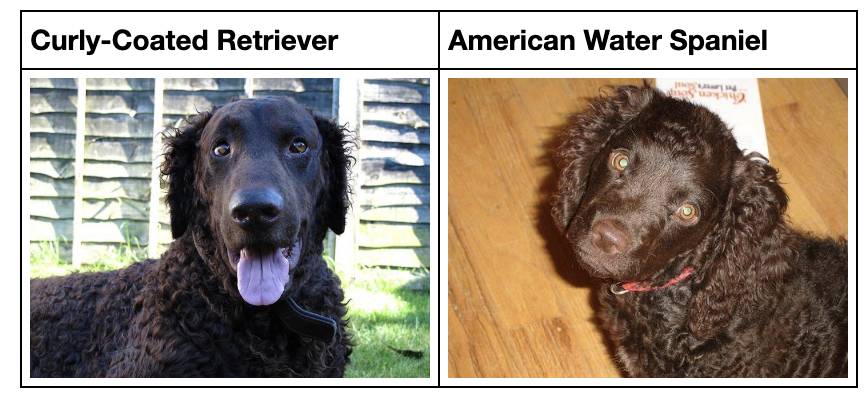
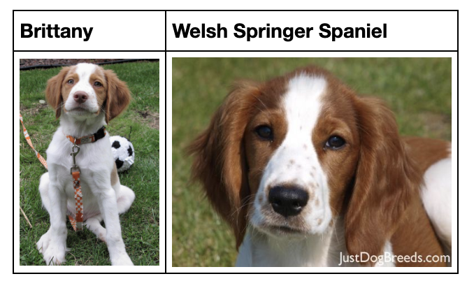It’s challenging even for humans to identify a dog breed

Let’s look at some of our data. Our example indicates that accurately identify a dog breed is challenging, even for humans. There are numerous other real-world factors that can affect our model:

• Lighting condition: different lightings change how colors are displayed

• Object orientation: our dogs can help many different poses

• Picture frame: a close-up portrait frame is very different than full body-shot

• Missing features: not all features of a dog is shown in a photo

As such, it has been impossible for traditional methods to advance in computer vision tasks. Let’s see what we can do with CNN and transfer learning.

Create a model of your own

Model architecture

Creating a CNN is straightforward with Keras. You can define your model architecture with the following code.

    from keras.layers import Conv2D, MaxPooling2D, GlobalAveragePooling2D
    from keras.layers import Dropout, Flatten, Dense
    from keras.models import Sequential

    model = Sequential()
    model.add(Conv2D(filters=16, kernel_size=2, padding='same',activation='relu',input_shape=(224,224,3)))
    model.add(MaxPooling2D())
    model.add(Conv2D(filters=32, kernel_size=2, padding='same',activation='relu'))
    model.add(MaxPooling2D())
    model.add(Conv2D(filters=64, kernel_size=2, padding='same',activation='relu'))
    model.add(MaxPooling2D())
    model.add(GlobalAveragePooling2D())
    model.add(Dense(133,activation='softmax'))

    model.summary()

Our primitive model architecture has an input layer with a shape of 224x224x3. The inputs are then fed to two convolutional layers, followed by a max-pooling layer (for downsampling). The outputs are then fed to a global average pooling layer to minimize overfitting by reducing the number of parameters. The output layer returns 133 probabilities for our breeds.

Image credit: Visualization of pooling layers such as MaxPooling and AveragePooling

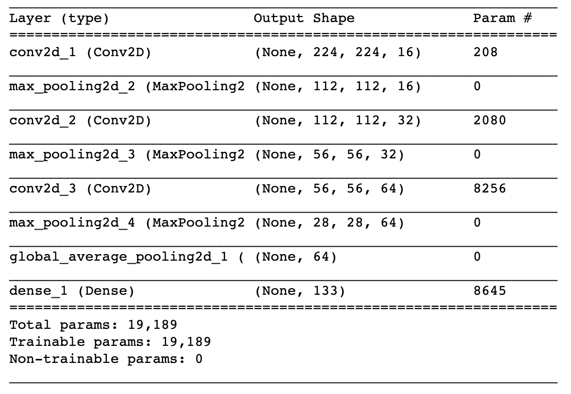Our primitive model summary

Metrics

In this project, our goal is to predict the breed of our dog image correctly. As such, we use accuracy as the measurement of choice to improve our model after each iteration. Accuracy is simply how many times our model predicts the dog breed correctly.

Compile and train the model

Our model will then need to be compiled. We use rmsprop as our optimizer, categorical_crossentropy, as our loss function and accuracy as our metric.

    model.compile(optimizer='rmsprop', loss='categorical_crossentropy', metrics=['accuracy'])

We can then train the model with the following codes:

    from keras.callbacks import ModelCheckpoint

    epochs = 5

    checkpointer = ModelCheckpoint(filepath='saved_models/weights.best.from_scratch.hdf5',
                                   verbose=1, save_best_only=True)

    model.fit(train_tensors, train_targets,
              validation_data=(valid_tensors, valid_targets),
              epochs=epochs, batch_size=20, callbacks=[checkpointer], verbose=1)

With five epochs and about eight minutes, we have achieved an accuracy of 3.2297%, better than random guessing (1/133 = 0.75%).

While our model performs much better than random guessing, a model of 3.2297% is no use in reality. Training and tuning our model to achieve meaningful accuracy require a lot of time, a large dataset, and high computing resources. Fortunately, we can use transfer learning to reduce training time without sacrificing accuracy.

Create a model using transfer learning

Obtain bottleneck features

Keras offers the following pre-trained state-of-the-art architectures that you can use in minutes: VGG-19, ResNet-50, Inception, and Xception. In this project, we will use ResNet-50, but you can try out other architecture on your own. The following code downloads the pre-trained model and load bottleneck features.

    import requests
    url = 'https://s3-us-west-1.amazonaws.com/udacity-aind/dog-project/DogResnet50Data.npz'
    r = requests.get(url)

    with open('bottleneck_features/DogResnet50Data.npz', 'wb') as f:
        f.write(r.content)

    bottleneck_features = np.load('bottleneck_features/DogResnet50Data.npz')
    train_Resnet50 = bottleneck_features['train']
    valid_Resnet50 = bottleneck_features['valid']
    test_Resnet50 = bottleneck_features['test']

Model architecture

With the pre-trained ResNet-50 model, we create our fully-connected (FC) layers with the following codes. We also add two dropout layers to prevent overfitting.

    Resnet50_model = Sequential()
    Resnet50_model.add(GlobalAveragePooling2D(input_shape=train_Resnet50.shape[1:]))
    Resnet50_model.add(Dropout(0.3))
    Resnet50_model.add(Dense(1024,activation='relu'))
    Resnet50_model.add(Dropout(0.4))
    Resnet50_model.add(Dense(133, activation='softmax'))
    Resnet50_model.summary()

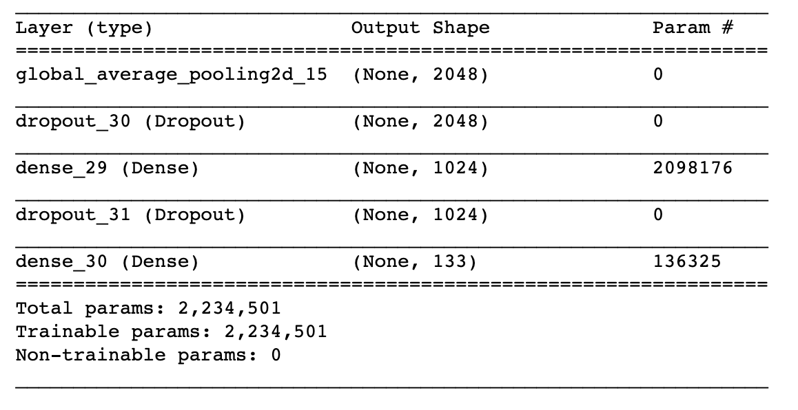Our model architecture using transfer learning looks like this

Model performance

Using transfer learning (ResNet-50), with twenty epochs and less than two minutes, we have achieved a test accuracy of 80.8612%. What a fantastic improvement over our primitive model.

Using the model described above, I have created a small command-line app. If you input a picture of a dog, the app will predict the breed. If you input a human image, say one of your friends, the app will predict the closest match dog breed. If no dog or human presented, the app would output an error. You can follow the instructions in the README.md file on my GitHub repo.

Conclusion

In this project, I walk you through some core concepts that you need to know to build your first computer vision project. I explained how computers understand images, briefly going over what a neural network, convolutional neural network, and transfer learning are.

We also built and trained a CNN architecture from scratch as well as apply transfer learning to vastly improve our model’s accuracy from 3.2% to 81%. While doing the project, I was very impressed at how you can use transfer learning to increase accuracy while reducing training time significantly. Here are some predictions of our models:

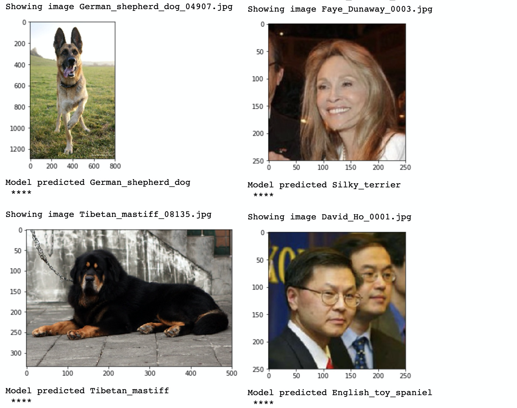Some predictions of our model

Future improvements

If I have more time, here are several future developments for this project:

• Augment data: The current implementation only takes in standard images as input. As a result, the model might not be robust enough in a real-world context. I can augment the training data to make our model less prone to over-fit. I can do so by randomly cropping, flipping, rotating the training data to create more training samples.

• Tune model: I can also tune the model hyperparameters to achieve better accuracy. Some potential hyperparameters for tuning include optimizer, loss function, activation function, model architecture, etc. I can also use GridSearch from Sklearn with Keras.

• Try other models: In this project, I have tried training the model on VGG-16 and ResNet-50. One next step could be to try training the models using different architectures as well as changing the architect of our fully connected layers.

• Create a web/mobile app: I can also create a web app or a mobile app using this model for fun.

Thank you for reading, I hope you learn something :)