Build your first data warehouse with Airflow on GCP
in Blog
Airflow has grown to be an essential part of my toolset as a data professional. After my previous post, many people reached out to me, asking about how to get started learning Airflow. As with many things else, I believe that the best way to get started learning something is by doing.
In this project, we will build a data warehouse on Google Cloud Platform that will help answer common business questions as well as powering dashboards. You will experience first hand how to build a DAG to achieve a common data engineering task: extract data from sources, load to a data sink, transform and model the data for business consumption.
Check out my previous post if you don’t know what Airflow is or need help setting it up. Getting started with Airflow locally and remotely Airflow has been around for a while, but it has gained a lot of traction lately. So what is Airflow? How can you use…towardsdatascience.com
Why Google Cloud Platform?
The short answer is BigQuery. While there are many data warehouse solutions on the market, either as a cloud provider’s solution or as an on-premise deployment, my experience with BigQuery has been the most pleasant.
Cost
Firstly the pricing model is straight forward and affordable at a small or large scale. Instead of paying for an always-on instance (winking at you, Redshift), you spend $20 per month per terabyte in storage cost and $5 for every terabyte scanned every time you query.
Let say your data set is 200GB in size, which is reasonably large for a structured data set. You will pay only $2 per month for storage costs. In term of query cost, you will not be spending a fortune either since BigQuery is a columnar database, which means instead of scanning the whole table every time you query, the engine will only scan your selected columns, which depends on the way you structure your data warehouse, is a significant cost-saving. A rough estimate is that you will scan over all your data about 50 times a month, which is equivalent to scanning 10TB and sets you back $50.
So with a reasonably sized structured data warehouse, you are looking at only $52 per month, compared to the cheapest always-on RedShift instance $146 per month. If the lowest tier of Redshift does not suit your needs, you are looking at paying about $2,774 a month, whether you utilize your data warehouse intensely or not. To me, the on-demand pricing of BigQuery is more desirable.
Ease of use
This is more of a personal opinion than a hard fact, but I think GCP is more user friendly than AWS. Operations like maintaining permissions or querying data from your browser are generally more user-friendly in GCP. Plus, BigQuery automatically does many of the optimizations to speed up your query behind the scene for you.
Business objective
Before setting out to do any data warehousing project, you should have a well-defined business problem that you are trying to solve. For this project, I chose the I94 Immigration data provided by the U.S. government, along with several complementary datasets.
Say you are working as a Data Engineer for the Immigration department of the United States. Your boss approaches you, saying that the current approach to analyzing immigration patterns is manual, time-consuming, and error-prone. He wants you to come up with a solution that would make the analytics process easier, faster, and scalable.
The data warehouse will help US officials to analyze immigration patterns to understand what factors drive people to move.
The dataset
You can choose any free data sources for this project and follow along. You can find many useful datasets on Kaggle or Google Dataset search. Here are the datasets used in this project.
I94 Immigration Data: This data comes from the U.S. National Tourism and Trade Office.
I94 Data dictionary: Dictionary accompanies the I94 Immigration Data
World Temperature Data: This dataset came from Kaggle.
U.S. City Demographic Data: This data comes from OpenSoft. You can read more about it here.
Airport Code Table: This is a simple table of airport codes and corresponding cities. It comes from here.
Data modeling
From the raw data, our next step would be to design a data model for the data warehouse. The data model should be closely tied to the business objectives and what you are trying to answer.
I designed the following model according to the star-schema principal with one fact table and seven dimensions tables.
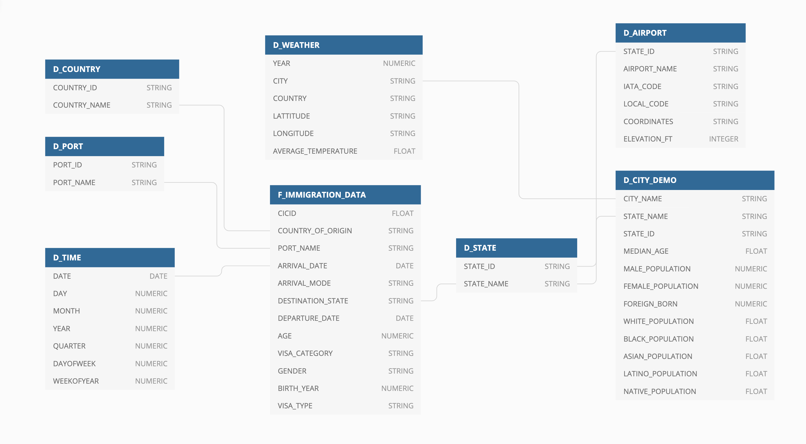 The data model for our data warehouse
F_IMMIGRATION_DATA: contains immigration information such as arrival date, departure date, visa type, gender, country of origin, etc.
D_TIME: contains dimensions for date column
D_PORT: contains port_id and port_name
D_AIRPORT: contains airports within a state
D_STATE: contains state_id and state_name
D_COUNTRY: contains country_id and country_name
D_WEATHER: contains average weather for a state
D_CITY_DEMO: contains demographic information for a city
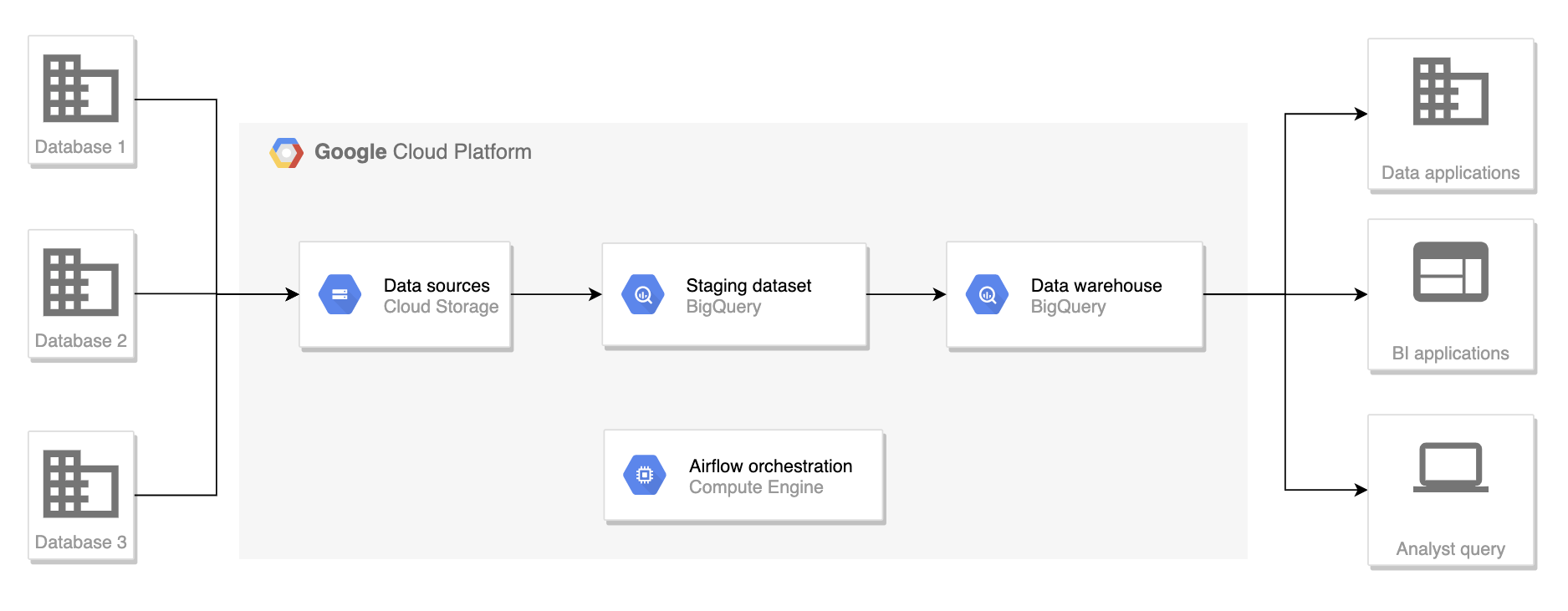
Architecture
The architecture for this project
We will skip the extract step from different databases and assume that we have all of our data in Google Cloud Storage (GCS) for this project.
GCS will act as the data sources where all raw files are stored. Data will then be loaded to staging tables on BigQuery. The ETL process will take data from those staging tables and create data warehouse tables.
An Airflow instance is deployed on a Google Compute Engine or locally to orchestrate the execution of our pipeline.
Here are the justifications for the technologies used:
Google Cloud Storage: act as our data sources, vertically scalable.
Google Big Query: act as a database engine for data warehousing, data mart, and ETL processes. BigQuery is a serverless solution that can efficiently and effectively process petabytes scale datasets.
Apache Airflow: orchestrate the workflow by issuing CLI commands to load data to BigQuery or SQL queries for the ETL process. Airflow does not have to process any data by itself, thus allowing our pipeline to scale.
Set up the infrastructure
To run this project, you should have a GCP account. You can create a new Google account for free and receive $300 in credits. With the free credits and free tier, you should get through this project without paying anything. You can refer to my previous article here to set up Airflow on a Google Compute Engine instance and run my code here to easily create the necessary cloud resources for the project.
Otherwise, you can use the GCP UI to create a GCS bucket, BigQuery datasets, and BigQuery tables.
Create a project on GCP
Enable billing by adding a credit card (you have free credits worth $300)
Navigate to IAM and create a service account
Grant the account project owner. It is convenient for this project, but not recommended for a production system. You should keep your key somewhere safe.
You can copy the data to your bucket by running the following:
gsutil cp -r gs://cloud-data-lake-gcp/ gs://{your_bucket_name}
Check out my GitHub repo for more info.
Data pipeline
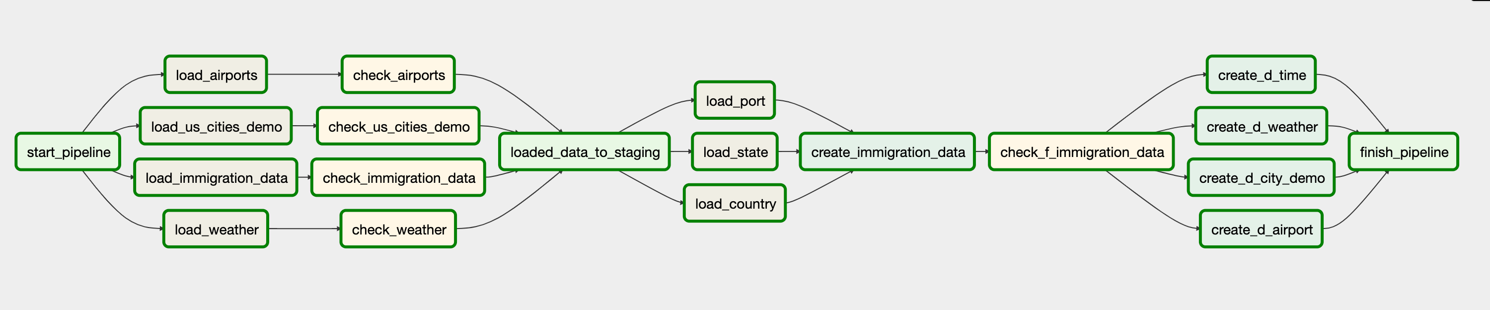 The data pipeline
With all the designing and setting up out of the way, we can start with the actual pipeline for this project. You can reference my GitHub repo for the code used below. tuanchris/cloud-data-lake This project creates a data lake on Google Cloud Platform with main focus on building a data warehouse and data…github.com
A DummyOperator start_pipeline kick off the pipeline followed by four load operations. Those operations load data from GCS bucket to BigQuery tables. The immigration_data are loaded as parquet files while the others are csv formatted. There are operations to check rows after loading to BigQuery.
Next, the pipeline loads three master data object from the I94 Data dictionary. Then the F_IMMIGRATION_DATA table is created and check to make sure that there are no duplicates. Other dimension tables are also created, and the pipelines finish.
Import airflow libraries
The first thing you should do to define a new dag is to import required libraries from Airflow. We should import DAG from Airflow, along with any operators that you wish to use. You can read the Airflow document to find out what an operator does and how to use one.
Different operators can have the same parameters, and defining all the same parameters every time you use an operator is repetitive. That’s why you should define a default set argument that will be passed to all of your tasks.
Define the DAG
The next thing to do is define a DAG. You should give it a unique name, a start date, and a schedule_interval. You can also pass in the default arguments defined above to your DAG.
You can use Airflow Variable to pass in variables instead of defining them in the DAG definition code like me below. The rule of thumb is for variables that you will change often, use Airflow variables. Otherwise, you can get away with using standard Python variables. Keep in mind that you should not define tons of Airflow variables; otherwise, you will likely overload the metadata database of Airflow.
Define load tasks from GCS
For four of our datasets, we will use the GoogleCloudStorageToBigQueryOperator to load data from GCS to BigQuery. You can read the Airflow document to find out more about how you should pass in variables to the operator.
In our example, we load the dimension files in the CSV format and the immigration data in the parquet format. Notice that for CSV files, you should provide a schema to ensure that data are loaded in the expected format. You don’t need to do so with parquet format since a parquet file already come with a schema.
Define data check
After we load the data to BigQuer, we should check whether our previous tasks run as expected. We can do that by merely checking the row count of our tables to verify if any row exits. You can implement a more sophisticated data quality check here according to your business needs.
Create fact and dim tables
With the staging data loaded and checked in the staging dataset, I use the BigQueryOperator to execute SQL queries to transform and load fact and dim tables.
Notice that I pass in parameters in my queries in place of datasets and tables. This makes it easier when moving between development and production environments. Check out my SQL queries in the GitHub repo to find out what logic I used for the transformation.
Define task dependencies
Finally, we have to define task dependencies, meaning which tasks are dependent on one another. You can do that using the » or « operator. You can also use a list to group multiple tasks.
The outcome
After all these steps, you will have a data warehouse to present to your boss.
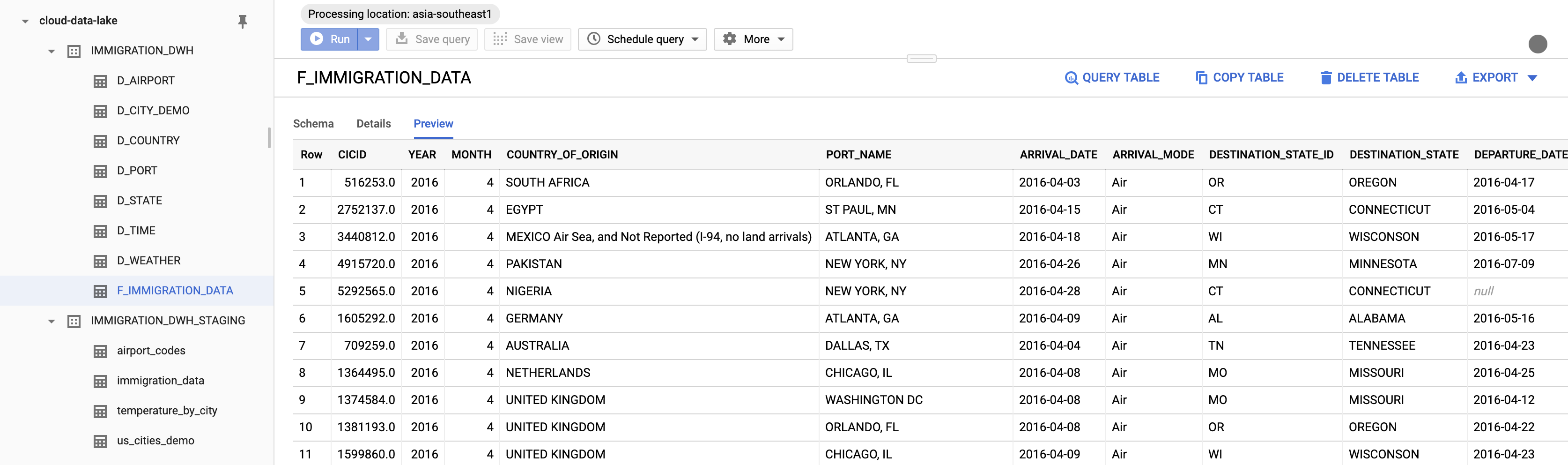 Our data warehouse
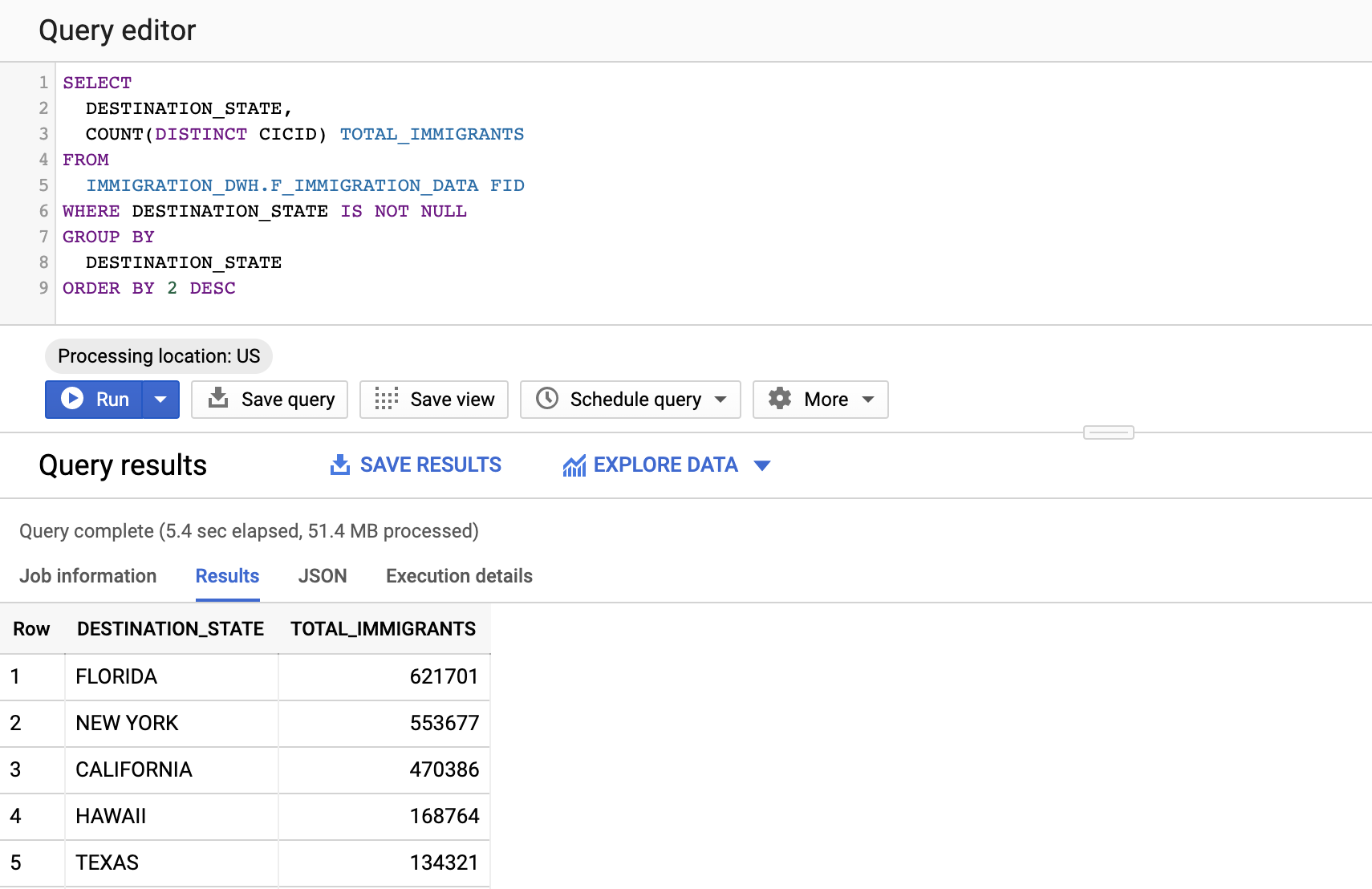
Let’s take our data warehouse for a run. Let’s see which States have the highest number of immigrants. It looks like Florida had the highest number of immigrants in our dataset, followed by New York and California.
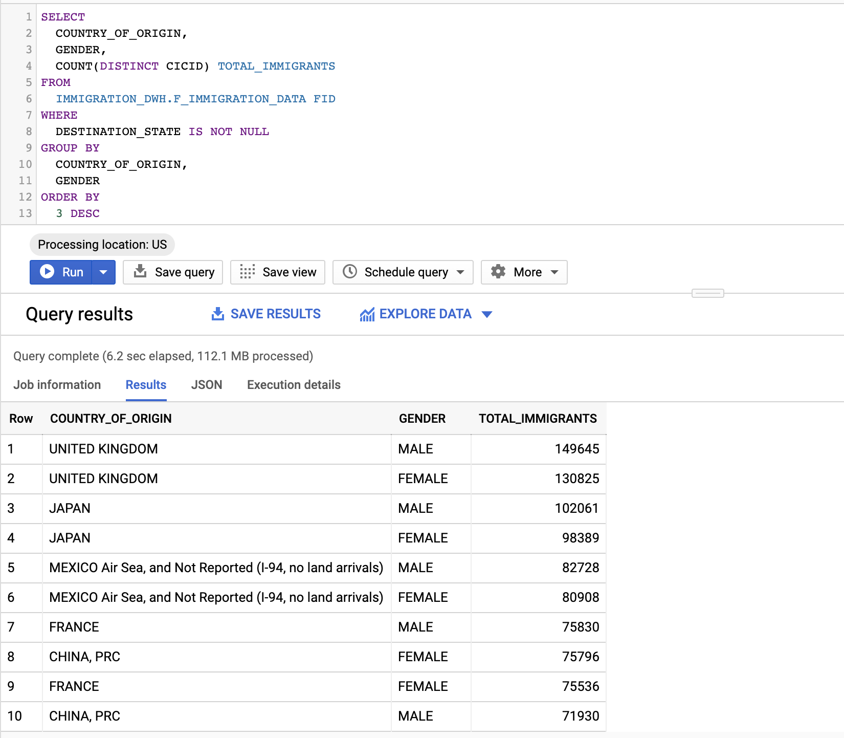
How about who is migrating to the U.S., and what are their genders?
Clean up
Remember to turn off your Airflow instance/delete unused resources to avoid unwanted charges.
Summary
In this article, I walked through the many steps of designing and deploying a data warehouse in GCP using Airflow as an orchestrator. As you can see, it is a lengthy and complicated process, so I cannot cover everything in one article.
I hope you have a better understanding of what a Data Engineer does and can put this knowledge to use.
Happy learning!